High Level Steps
- Import the Data
- Clean the Data
- Split the Data into Training/Test Sets (80% training/20% testing)
- Create a Model - select an algorithm
- Train the Model
- Make Predictions
- Evaluate and Improve
Libraries and Tools
| Library | Purpose |
|---|---|
| NumPy | NumPy offers comprehensive mathematical functions, random number generators, linear algebra routines, Fourier transforms, and more. |
| Pandas | Pandas is a fast, powerful, flexible and easy to use open source data analysis and manipulation tool. |
| MatPlotLib | Matplotlib is a comprehensive library for creating static, animated, and interactive visualizations in Python. |
| SciKit-Learn | Simple and efficient tools for predictive data analysis · Accessible to everybody, and reusable in various contexts |
| Jupyter | The Jupyter Notebook App is a server-client application that allows editing and running notebook documents via a web browser. |
| Anaconda | Anaconda is a distribution of the Python and R programming languages for scientific computing, that aims to simplify package management and deployment. |
Getting Started
Install Anaconda
https://www.anaconda.com/products/individual
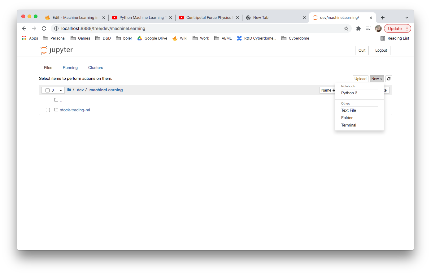
Start a jupyter notebook
$ jupyter notebook
Create a new Python3 notebook
Import a Dataset
We can get some sample datasets from kaggle.com - https://www.kaggle.com/
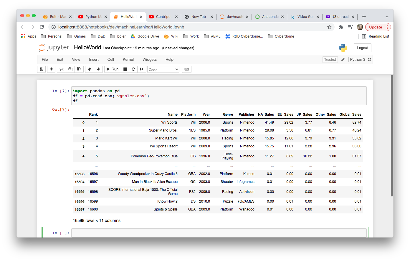
From our Jupyter notebook, we are going to import a downloaded CSV.
import panda as pd
df = pd.read_csv('vgsales.csv')
df
The pd.read function returns a DataFrame object
Dataframe Functions:
Interesting DataFrame functions:
| Method | Description | Example |
|---|---|---|
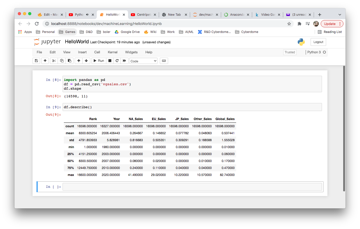
| shape | returns dimensions of dataset | df.shape (16598, 11) |
| describe | returns useful statistics about our data | df.describe() (see above image) |
| values | returns your data |
Jupyter Shortcuts
| Shortcut | Mode | Key | Description |
|---|---|---|---|
| Add Cell Above | Command | a | |
| Add Cell Below | Command | b | |
| Delete Current Cell | Command | dd | |
| Run current Cell and Stay in Cell | Command/Edit | <CTRL><ENTER> | Run Commands in cell without adding a cell below. |
| Autocompletion | Edit | <TAB> | Get methods for object |
| Method Documentation | Edit | <SHIFT> <TAB> | Get information on method |
| Make Comment | Edit | <CMD> / | Comment/UnComment |
Real Example
Import the data
import pandas as pd
df = pd.read_csv('music.csv')
df
Spit the Data
Create input and output data sets. X = input, y = output.
Since we want to predict the type of music based on age and sex, we create our input data as X and our output as y.
import pandas as pd
df = pd.read_csv('music.csv')
X = df.drop(columns="genre")
y = df["genre"]
y
Train and Do a Prediction
import pandas as pd
from sklearn.tree import DecisionTreeClassifier

df = pd.read_csv('music.csv')
X = df.drop(columns="genre")
y = df["genre"]

model = DecisionTreeClassifier()

# train model
model.fit(X,y)

# predict
# 21 year old male and 22 year old female
predictions = model.predict([[21,1],[22,0]])
predictions
In the above example, we used 100% of the data for training and 0 for testing our model.
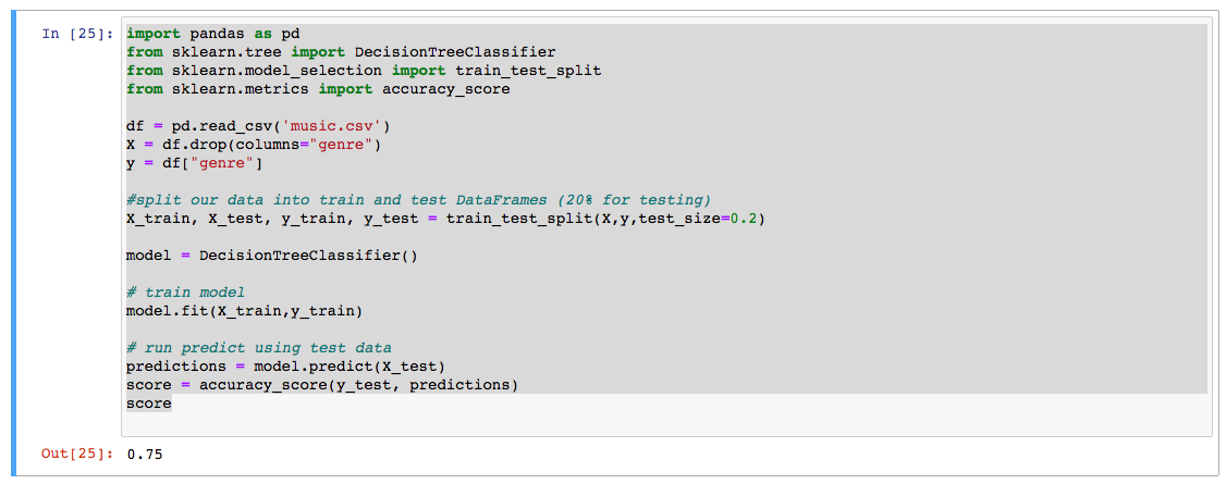
Testing our Model
import pandas as pd
from sklearn.tree import DecisionTreeClassifier
from sklearn.model_selection import train_test_split
from sklearn.metrics import accuracy_score

df = pd.read_csv('music.csv')
X = df.drop(columns="genre")
y = df["genre"]

#split our data into train and test DataFrames (20% for testing)
X_train, X_test, y_train, y_test = train_test_split(X,y,test_size=0.2)

model = DecisionTreeClassifier()

# train model
model.fit(X_train,y_train)

# run predict using test data
predictions = model.predict(X_test)
score = accuracy_score(y_test, predictions)
score
Model Persistence
Saving a Trained Model
import pandas as pd
from sklearn.tree import DecisionTreeClassifier
from sklearn.model_selection import train_test_split
from sklearn.metrics import accuracy_score
import joblib

df = pd.read_csv('music.csv')
X = df.drop(columns="genre")
y = df["genre"]

#split our data into train and test DataFrames (20% for testing)
X_train, X_test, y_train, y_test = train_test_split(X,y,test_size=0.2)

model = DecisionTreeClassifier()

# train model
model.fit(X_train,y_train)

# run predict using test data
# predictions = model.predict(X_test)
# score = accuracy_score(y_test, predictions)

#save our model
joblib.dump(model,"music-recomender.joblib")
Predictions from a Saved Model
import joblib

#load our model
model = joblib.load("music-recomender.joblib")

# run predict using test data
predictions = model.predict([[20,1],[21,0]])

predictions
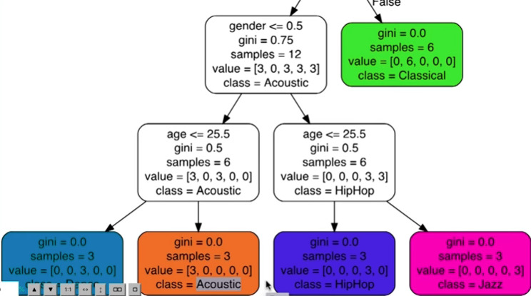
Visualizing Decision Trees
import pandas as pd
from sklearn.tree import DecisionTreeClassifier
from sklearn import tree

df = pd.read_csv('music.csv')
X = df.drop(columns="genre")
y = df["genre"]

model = DecisionTreeClassifier()

# train model
model.fit(X,y)

# export graph of data in dot format
tree.export_graphviz(model,out_file='music_recomender.dot',
                    feature_names=['age','gender'],
                    class_names=sorted(y.unique()),
                    label='all',
                    rounded=True,
                    filled=True)
This will output our .dot file. We just need to pull it into VSCode with dot plugin to visualize it.
References
| Reference | URL |
|---|---|
| Python Machine Learning Tutorial (Data Science) | https://www.youtube.com/watch?v=7eh4d6sabA0 |